← All skills

Skill

C++

Systems programming in modern C++. I wrote Achilles, my rigid-body simulator, in C++20 from the SIMD layout to the contact solver, plus ARUW's odometry and path tracking and the OpenArm controllers.

13 log entries3 projects

AchillesBest example

Collision response

Code

Also shows: Kinematics & Dynamics

Detecting contacts is only half the battle; working out what happens next is the rest. Once accelerations and contacts are known, the solver adjusts the accelerations so bodies respect their contacts. It uses a "soft contact" model in which each contact acts like a stiff spring-damper, pushing harder the deeper and faster two bodies collide. Friction follows Coulomb's law, whose cone of allowed forces is approximated by a four-sided pyramid of push-only edges, letting bodies grip or slide. Each frame, the solver minimizes

½ (a − a₀)ᵀ M (a − a₀) + Σᵢ ½ Dᵢ (Jᵢ a − a_ref,ᵢ)²,

staying close to the unconstrained acceleration a₀ while penalizing contact violations. It warm-starts from the previous frame's solution when that costs less, then runs a fixed 20 conjugate-gradient iterations to suit SIMD and GPUs, never building the mass matrix. The corrected acceleration then goes to the integrator.
Real time, rendered by the Achilles viewer: semi-implicit Euler at a 2 ms step.
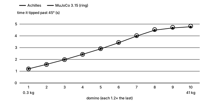
Chart of the time each of the ten dominoes tipped past 45 degrees, from 1.2 seconds for the first to 4.8 seconds for the last. Achilles' points sit inside MuJoCo's rings for every domino.
The same scene in MuJoCo 3.15: each domino tips within 56 ms of MuJoCo's time, and all ten come to rest within 0.3° of MuJoCo's angles.

Achilles

SIMD: eight robots per instruction

Pull request

Also shows: Performance & SIMD

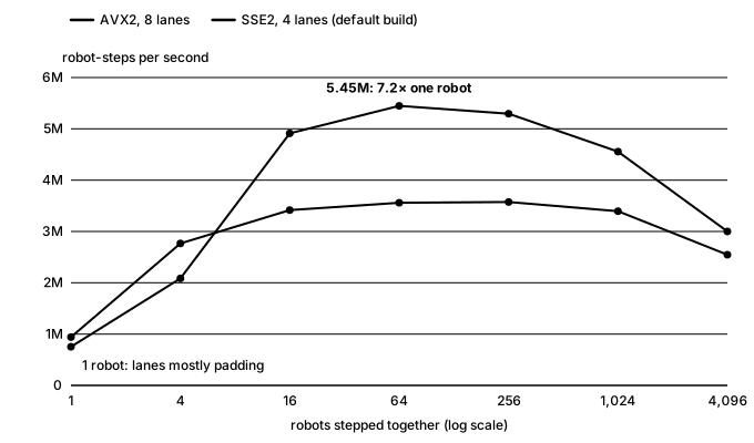
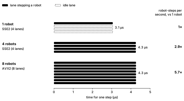
V3 replaces V2's Eigen with my own spatial algebra on xsimd, and stores every field as a structure of arrays: each component of each field, say the x angular velocity of every joint, is its own contiguous, aligned array. Joints are sorted by their depth in the tree, and each group of SIMD lanes holds joints at the same depth. With many copies of one robot, that puts the same joint of different robots side by side, so one instruction can load, update or store a quantity for eight robots at once (eight lanes with AVX2, four in the default SSE2 build). A Valgrind trace of the compiled binary confirms it: 88.9% of all accesses to simulation data are whole, aligned 8-lane vector loads or stores. The payoff is that filling the lanes is nearly free. On a seven-link arm, one robot takes 3.1 µs per step, while eight robots in the 8-lane build take 4.3 µs, 5.7× the robot-steps per second.

Three bars of SIMD lanes showing the time for one step of a seven-link arm: one robot in the 4-lane build takes 3.1 microseconds with three lanes idle; four robots fill the lanes in 4.3 microseconds, 2.9 times the robot-steps per second; eight robots in the 8-lane AVX2 build take 4.3 microseconds, 5.7 times
One step of a seven-link arm on one CPU core, best of 18 runs. Batched runs also step one shared fixed root.
Line chart of robot-steps per second against robots stepped together, seven-link arm. With one robot, 8-lane AVX2 does 0.75 million and 4-lane SSE 0.94 million. AVX2 climbs to 5.45 million at 64 robots, 7.2 times its one-robot rate; SSE levels off near 3.6 million.
The same effect across batch sizes: throughput climbs until the lanes are full.

Achilles

Beating MuJoCo on throughput

Benchmark code

Also shows: Simulation (MuJoCo)Performance & SIMD

To see where V3 stood, I benchmarked it against MuJoCo 3.15 on the same arm scenes, converted from the same .arow files, at the same 2 ms step, single-threaded on my laptop (Intel Core Ultra 9 285H). Batched across SIMD lanes, Achilles steps a seven-link arm 3.3× faster than MuJoCo's best single-threaded mode, reaching 5.45 million robot-steps per second at 64 robots. In double precision, MuJoCo's own, Achilles is still 1.5–1.6× faster at most batch sizes, and its results match MuJoCo's to about one part in 10¹¹. The one loss is a single seven-link arm, where most SIMD lanes sit empty (0.97×).

Line chart of speed relative to MuJoCo by number of links. V2 with one robot falls from 1.1× at one link to 0.48× at eight. V3 with one robot is 2.8×, 2.1×, 1.6× and 0.97× at one, two, three and seven links. V3 with 64 robots batched is 2.7×, 2.6×, 3.0× and 3.3×.
Each version timed against MuJoCo on the same machine, in its own benchmark: V2 against MuJoCo 3.3 (no gravity, 1 ms step), V3 against MuJoCo 3.15 (2 ms step).
The same double pendulum in Achilles and MuJoCo, matching out to 8 seconds. Same scene and start, both RK4 at a 2 ms step.

Achilles

Dynamics: the Articulated Body Algorithm

Pull request

Also shows: Kinematics & DynamicsSimulation (MuJoCo)

V2's dynamics were wrong in ways only a reference could show: brought back to life next to MuJoCo, a one-link arm swung exactly 4× too fast (it used the free-body inverse inertia, dropping the parallel-axis term), and a two-link arm moved in the wrong shape. V3 runs the full Articulated Body Algorithm, with Coriolis and centrifugal bias terms, parent-to-body transforms and gravity as a fictitious base acceleration, and steps it forward with semi-implicit Euler, the same default MuJoCo uses. Here all three drive the same arm with the same shoulder torque and no gravity, since V2 never had any. V3 stays within 3×10⁻⁵ rad of MuJoCo for all 4 seconds, while V2 has swung the shoulder 4.5 times as far and folded the elbow forward instead of letting it trail behind.

The demo arm with a constant 0.1 N·m on the shoulder, none on the elbow and no gravity, semi-implicit Euler at 1 ms. All three are drawn by MuJoCo's renderer, since V2 never had one; the yellow trail is the forearm tip's last second.

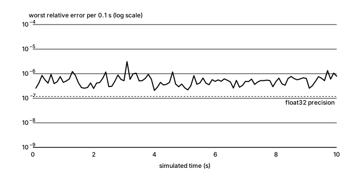
MuJoCo is only a reference, so I also checked V3 against an exact answer. A double pendulum is chaotic and has no closed-form trajectory: two simulations that differ by a single rounding error eventually go completely different ways. Its equations of motion do have a closed form, though. Lagrangian mechanics reduces them to a 2×2 linear system that gives the exact joint accelerations at any given position and velocity. I derived that system independently of the engine's code, then compared it with V3's accelerations at every state of a 10-second run. Because each state is checked on its own, errors can't build up and chaos can't amplify them. The two agree to within 3×10⁻⁶, which is float32 round-off, and V3 matches MuJoCo to the same 3×10⁻⁶.

Log-scale chart over 10 seconds of a double pendulum: the worst relative error in Achilles' joint accelerations against the closed-form solution stays between about 2e-7 and 3e-6, just above the float32 precision line, with no growth over time
ABA against the closed-form solution at every state of a 10-second double-pendulum run.

Achilles

Collision detection

Pull request

Before contacts can be resolved, they have to be found, and that happens in two phases. Every body carries a single "sphere-swept box," a box whose surface is pushed outward by a radius, so one shape type covers spheres, capsules, boxes and rounded boxes. The broad phase cheaply narrows the search. Each frame, it wraps every body in a world-aligned bounding box and tests every pair for overlap. It skips pairs whose collision groups exclude each other and bodies directly joined by a joint. The narrow phase then examines only the remaining candidates. For each pair, it computes a contact normal and up to four contact points, each with a signed distance that turns negative once the shapes overlap. Contacts within a small margin are kept even before the shapes touch, so the solver can react early. Both phases treat every pair the same way and mask out irrelevant results instead of branching, which keeps them SIMD- and GPU-friendly.

Detection only, at quarter speed: white outlines are the collision shapes, magenta the contacts and normals the narrow phase finds each frame. Nothing pushes back yet, so the arms pass through.
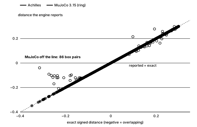
Scatter chart of reported against exact signed distance for 1,795 random shape pairs. Every Achilles point lies on the diagonal. MuJoCo's points also lie on it except for 86 box pairs, which scatter off the line
Each pair's distance as reported by each engine, against the exact answer. Sphere, capsule and box, all six combinations, from 0.35 overlapping to 0.3 apart.

Achilles

Integrators that hold energy

Commit

Also shows: Kinematics & Dynamics

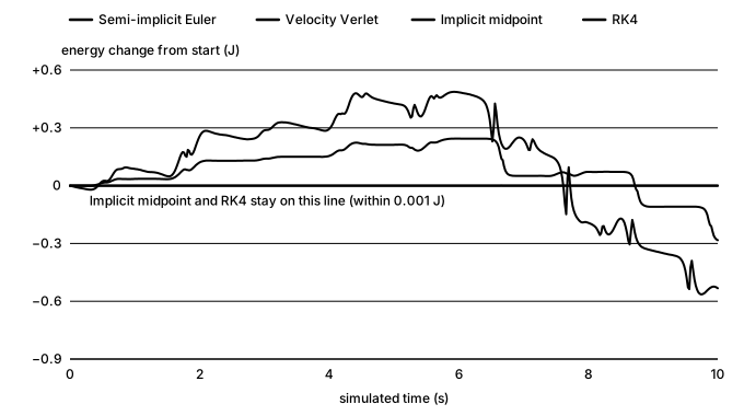
With the accelerations right, longer runs exposed the next problem: semi-implicit Euler drifts. A frictionless double pendulum should conserve energy, yet over 10 seconds at a 2 ms step Euler's total energy wanders by up to 0.56 J. Euler updates the velocity from the current acceleration, then moves the position with that new velocity, which is simple but only first-order accurate. Velocity Verlet splits the velocity update into two half-steps around the position update and recomputes the accelerations in between, halving the drift to 0.28 J. Its weakness is that velocity-dependent forces like Coriolis are evaluated at an estimated velocity. Implicit midpoint evaluates the dynamics at the average of the old and new states, making each step time-symmetric. Because the new state isn't known in advance, it iterates four times to converge, and it stays within 0.0006 J. RK4 instead samples the dynamics four times across the step and blends the results, reaching fourth-order accuracy and staying within 0.0001 J.

Chart of the change in total energy over 10 seconds for four integrators: semi-implicit Euler wanders between about −0.56 and +0.49 joules, velocity Verlet between about −0.28 and +0.24, and implicit midpoint and RK4 stay flat on the zero line
Energy should stay constant. Double pendulum released from horizontal, 2 ms step.

Advanced Robotics at UW

Kalman-filter odometry for three dead wheels

8-state filterSplit filters

Also shows: State estimation

Our robots know where they are from dead wheels: small unpowered tracking wheels with encoders that roll along the floor. When the engineer robot moved to new odometry pods with three of them, I rewrote the team's Kalman-filter odometry for them; I had taught myself Kalman filters from Kalman Filter from the Ground Up. The first version was one 8-state filter fusing the three wheels with the IMU. Its covariance between heading and the x and y motion turned out to be negligible, so I split it into three independent two-state filters, for x, y and heading, each updated by one measurement: every step now multiplies 2×2 matrices and divides by a number, instead of working through 8×8 matrices and inverting a 7×7 one, and the wheels alone turned out to be enough without the IMU. To tune it, I drove fixed paths (straight forward, straight sideways, spins and a square), logged the raw wheels, and replayed them offline to fit each pod's position, angle and wheel radius and the filter's noise, checking the result against the IMU's heading. Our target was under 10 cm of error over the engineer's path, the most our vision system could correct for, and the tuned odometry met it.

The engineer driving itself at competition, from the third cube pickup to its drop-off: the filter's own logged pose, replayed at real time from just before it moves.
Tuning offline: a logged 5 m sideways push, replayed through the filter as the pods move from their design values to the tuned ones. With one pod 2.7° off straight, the design values read the push as a 79° turn; tuned, it comes to 4.99 m and follows the path the IMU's heading gives, ending within 1° of it.

Advanced Robotics at UW

Path tracking: from pure pursuit to LQR

CodeThe LQR study

Also shows: Control systemsTechnical leadership

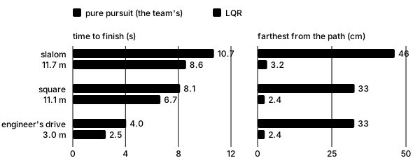
Our chassis followed paths with pure pursuit: aim at a point a fixed distance down the path and ramp the speed up toward it. The robot's accelerations stay implicit in that, so it has no idea how hard it can brake or how fast it can take a corner, and at speed it swings wide of turns and overshoots where it should stop. I proposed replacing it with path tracking that models those accelerations explicitly, and led the feature from idea to implementation: I wrote the design and gathered the resources behind it, from spline fitting and arc-length reparametrization to the Riccati equation and a study that found LQR tracks more accurately than pure pursuit. First, a cubic spline through the waypoints is reparametrized by arc length, the speed at each point is capped by its curvature, and a forward and a backward pass keep every speed-up and every stop within what the robot can deliver. Then an LQR tracks that profile on a world-frame model of the chassis, where its dynamics stay constant, and its force is rotated into the robot's frame. I designed it and built the framework; the comparison here runs the finished MVP against our pure pursuit in simulation.

The same slalom, the same simulated chassis and the same 2 m/s top speed: LQR (blue) against the team's pure pursuit (orange), in real time.
Bar charts for three paths: LQR finishes each sooner and stays within about 3 cm of the path, against 33 to 46 cm for pure pursuit
Three paths: LQR finishes 1.5 to 2.1 s sooner and stays within 3.2 cm of the path; pure pursuit strays up to 46 cm.

OpenDubs

Arm control: three impedance controllers, then a simpler one

Cartesian controlJoint and null-space control

Also shows: Impedance controlROS 2

Each arm is a 7-DOF OpenArm whose Damiao motors run their own impedance loop: the Thor sends position, velocity and torque targets with gains over CAN-FD, and each motor closes the loop itself. I measured the stock ROS 2 stack first. A goal is accepted in 2.55 ms, and with both arms holding one block, 47 ms passes between a command to one arm and the torque spike in the other (σ = 4.7 ms).

What I was after was axial compliance in Cartesian space: a gripper that holds firm along some axes and gives along others. I wrote three controllers with Pinocchio to get it (Cartesian, joint and null space). Pure Cartesian impedance gave that compliance, but it left the redundant elbow free to drift off the collision-checked path. The combined controller ran joint-space impedance and subtracted the Cartesian terms from it, keeping the axial compliance and control of the null space, but it was numerically unstable. The null-space controller worked, but I switched off it for the much lower latency of the motors' own impedance loops: in the end we gave up Cartesian compliance for speed.

What I settled on is simpler: the planned trajectory goes straight to the motors, plus gravity compensation at 500 Hz from Pinocchio's RNEA (the recursive Newton-Euler algorithm), with every goal checked against position and torque limits in both joint space and Cartesian space (through forward kinematics).

My Cartesian impedance controller on the robot: gravity compensation only (June 26), stiff in x and y but compliant in z and rotation, and stiff in x and y but compliant in rotation.
The four controllers in MuJoCo, built unchanged from their repos (faint arm: the plan). On the reaches the motors' own loop stays within about 2 cm of the plan while the others trail by 7 to 18 cm; near the straight arm the Cartesian one stays folded once pushed. Demo gains.

Achilles

A viewer drawn from the simulation's own state

Pull request

The viewer is a small OpenGL 3.3 program with GLFW as its only dependency. GLFW opens the window and also loads the handful of OpenGL functions the viewer needs. Every visible body is drawn from a single unit cube uploaded to the GPU once, then scaled and placed at that body's pose, with one draw call per body. The shading is simple directional lighting, and lines show the skeleton and a ground grid. You orbit the camera by dragging the mouse and zoom with the scroll wheel. The viewer reads only the simulation's render-only viz state, which is never stepped, so simulation ticks and drawn frames stay independent. Passing --headless skips the viewer entirely. Here, eight double pendulums are released 0.002 rad (about 0.1°) apart, and within a few seconds chaos sends each one its own way.

Recorded from the Achilles viewer, RK4 at a 2 ms step.

Achilles

V3: designing for performance

Commit

Also shows: Performance & SIMD

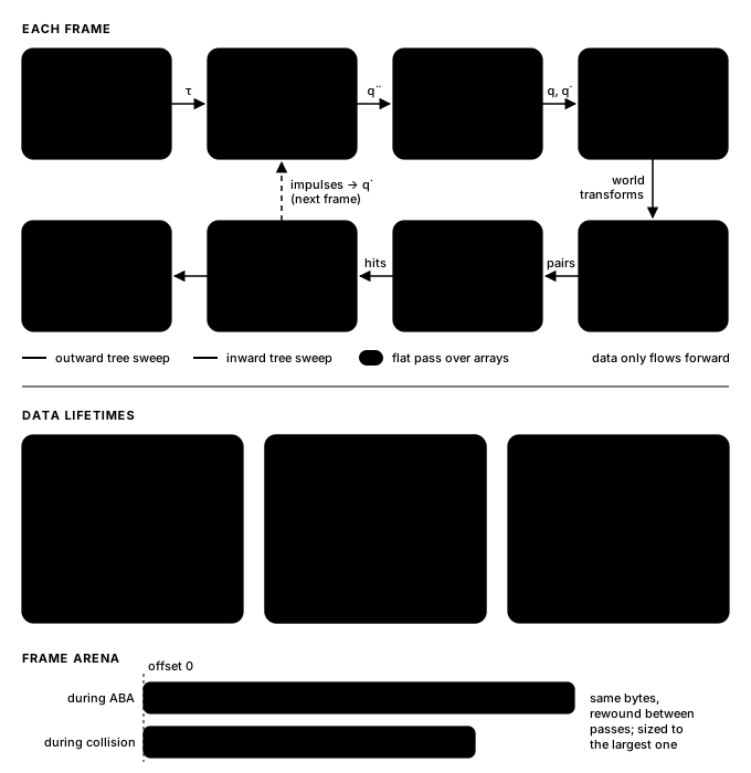
For V3, I wrote a full design document before writing any code. The target was concrete: simulate my club's six-robot arena of holonomic turret robots fast enough to train RL policies on a laptop CPU, since we don't have much GPU compute. Training takes millions of steps, so throughput was the goal, and V3 doubled as a performance learning exercise. One rule drove most decisions: only costs paid every frame matter. Only joint state, plus the contact solver's last solution, persists between frames. Everything else is either static data built at load time or scratch memory rebuilt each step and reused between passes. That rule became three pieces: fields; small operations that declare exactly which fields they read and write; and traversals that apply those operations across the joint tree, all checked at compile time. What the compiler can't check, the engine checks as it starts, and CI runs death tests confirming that a bad setup, like a model that doesn't fit its layout or an overflowing arena, stops it with a clear message instead of quietly corrupting a run. I kept V2's physically meaningful types but moved them into the math rather than the structure, so adding collisions or rendering meant adding passes instead of rewiring classes.

The V3 design: each frame runs eight passes in one direction (actuator torques, ABA forward dynamics, integration, kinematics, then broad phase, narrow phase, contact resolution and a debug render), and below it, which data is static, which persists between frames, and which is rebuilt each frame in a reused arena
V3 as designed. Collisions changed once I built them (see above).

Achilles

V2: types with physical meaning

Code

Also shows: Kinematics & Dynamics

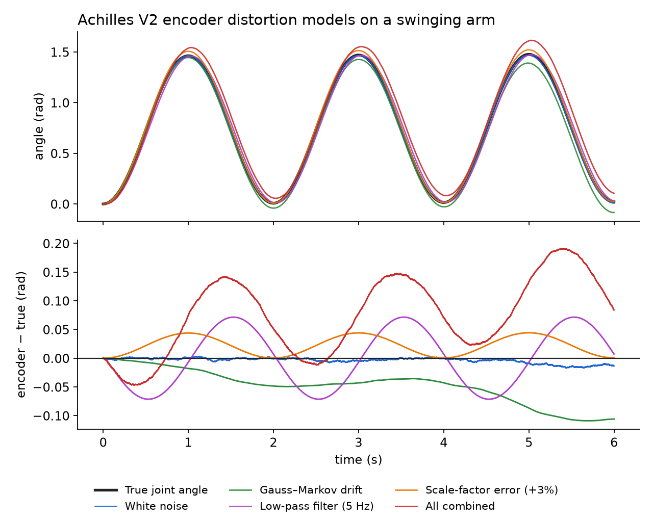
A major part of my design philosophy for V2 was making sure every quantity had a physical meaning. Velocity, acceleration and force each had their own type, and they only combined in physically valid ways: an acceleration integrated into a velocity, and an inertia turned a force into an acceleration. Every link, joint and actuator also carried a typed frame, so frames belonging to different kinds of objects couldn't be mixed up. The core of this model was the joint system. Each joint is defined by its motion subspace S, and a CRTP template turns that into fixed-size math, including the articulated-inertia step, so each joint type can be specialized. Because Achilles was meant to model my club's robots, I also built sensor models, starting with an encoder, with Gaussian noise, Gauss–Markov drift, a low-pass filter and scale-factor error. But when I started planning collisions and rendering, I realized the rigid architecture and very specific type flow had built me into a corner.

Simulated encoder readings on one swinging joint: the true angle, then readings with white noise, Gauss–Markov drift, a 5 Hz low-pass filter, a 3% scale-factor error, and all of them combined, which drifts visibly away from the truth over time
Each line is a V2 sensor model reading the same joint, from the April 14 code brought back to life.

Achilles

Actuators: closing the loop

Code

Also shows: Kinematics & DynamicsSimulation (MuJoCo)

Until now, every torque in Achilles came from the scene file, so a robot could fall or collide but never react. Actuators let a controller outside the simulation push on a joint every step. An actuator is a direction in its joint's frame, an angular one for a torque or a linear one for a force. Attaching it projects that direction onto the joint's free axes once, so applying an effort later costs only a few multiply-adds into the joint-torque field. The simulation never owns or loops over actuators: each one is a small handle into that field, which is now double-buffered. A controller writes one half while the step reads the other, and the halves swap at the start of every step. An effort therefore acts over exactly the next step and is then gone, so a stale command can never leak into a later frame. Here, two actuators tilt a plate to balance a ball. The controller never sees the ball directly, only through a simulated camera that reports its position 30 times a second, 50 ms late, with 2 mm of noise. The plate can tilt no faster than 3 rad/s, about what a hobby servo manages. The plate starts tipped with the ball on its high corner, and the controller has to catch the ball before it rolls off, center it, then roll it around a figure-8.

Real time, rendered by the Achilles viewer: semi-implicit Euler at a 4 ms step. The controller sees only the delayed, noisy camera; the simulation sees only the two pivot torques.

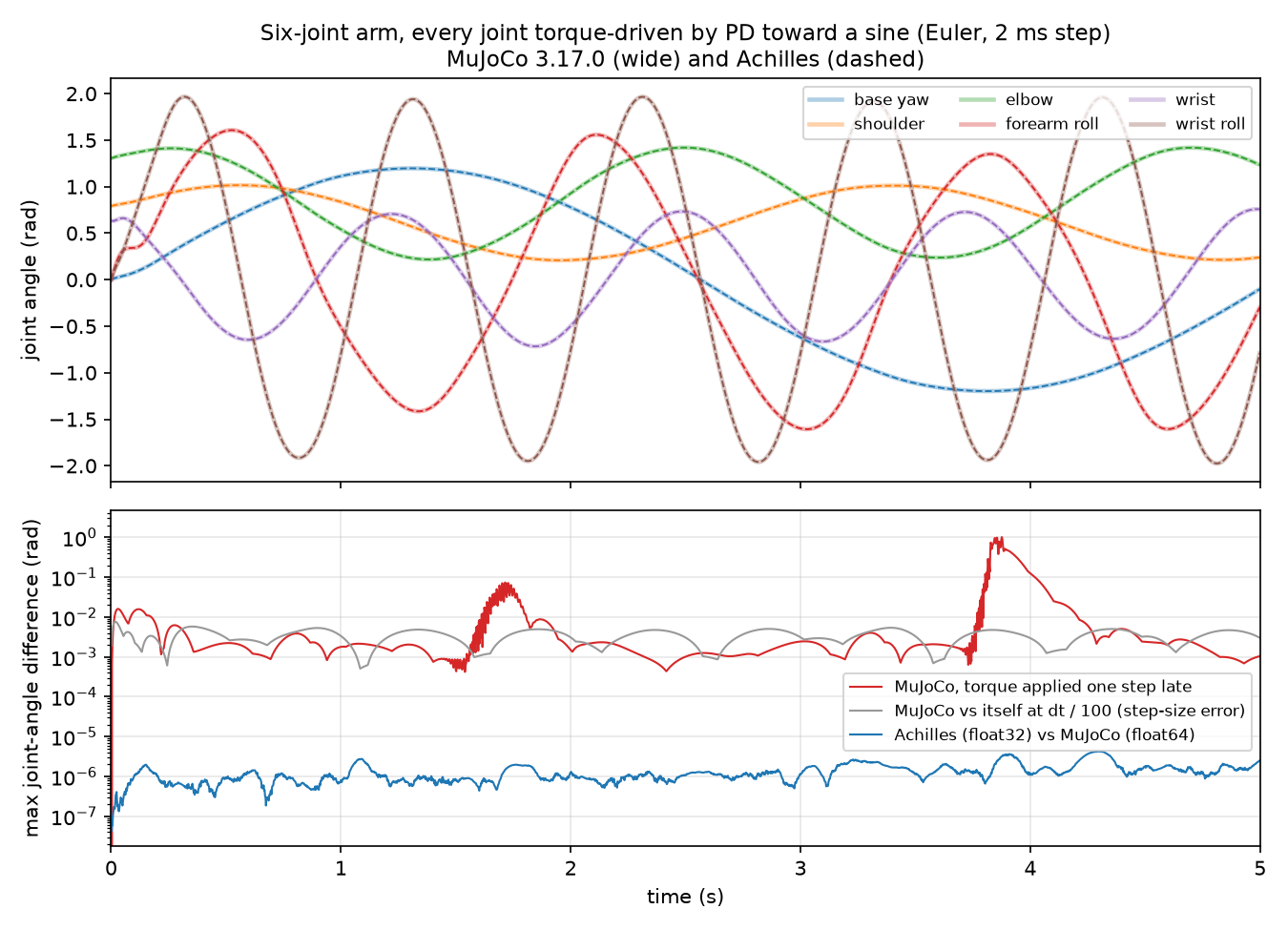
To check that an effort lands on exactly the step it was meant for, I drove a six-joint arm in both Achilles and MuJoCo 3.17. Every joint has an actuator running a PD loop toward its own sine wave, with torques up to 146 N·m. Both engines start from the same state at the same 2 ms step, and each step they read the joints, compute the torques, and apply them over the next step. Over 20 seconds, Achilles stays within 10⁻⁵ rad of MuJoCo under both semi-implicit Euler and RK4, which is float32 round-off, and the torques agree to 3×10⁻⁵. If the torques land one step late, MuJoCo ends up 1 to 2 rad away from its on-time run, so a timing slip would stand out by five orders of magnitude. The free-swinging arms in my throughput benchmark drifted apart after a few seconds because they're chaotic. Here the controller keeps pulling both arms back onto their targets, so the two engines stay together for the whole run.

Two charts over 5 seconds for a six-joint arm. Top: each joint's angle following its own sine wave, between about -2 and 2 rad, with Achilles drawn dashed on top of MuJoCo and the lines indistinguishable. Bottom, log scale: the largest joint-angle difference. Achilles against MuJoCo stays around one millionth of a radian; MuJoCo against itself at a 100 times smaller step stays near a thousandth; MuJoCo with torques applied one step late swings up to about 1 rad
Every joint torque-driven by PD toward a sine, semi-implicit Euler at a 2 ms step. Achilles in float32, MuJoCo in float64.