← All skills

Skill

Odometry

Tracking a robot's position from its own motion. Dead-wheel odometry for ARUW and optical-flow odometry for OpenDubs, both checked against ground truth.

2 log entries2 projects

Advanced Robotics at UWBest example

Kalman-filter odometry for three dead wheels

8-state filterSplit filters

Also shows: State estimationC++

Our robots know where they are from dead wheels: small unpowered tracking wheels with encoders that roll along the floor. When the engineer robot moved to new odometry pods with three of them, I rewrote the team's Kalman-filter odometry for them; I had taught myself Kalman filters from Kalman Filter from the Ground Up. The first version was one 8-state filter fusing the three wheels with the IMU. Its covariance between heading and the x and y motion turned out to be negligible, so I split it into three independent two-state filters, for x, y and heading, each updated by one measurement: every step now multiplies 2×2 matrices and divides by a number, instead of working through 8×8 matrices and inverting a 7×7 one, and the wheels alone turned out to be enough without the IMU. To tune it, I drove fixed paths (straight forward, straight sideways, spins and a square), logged the raw wheels, and replayed them offline to fit each pod's position, angle and wheel radius and the filter's noise, checking the result against the IMU's heading. Our target was under 10 cm of error over the engineer's path, the most our vision system could correct for, and the tuned odometry met it.
The engineer driving itself at competition, from the third cube pickup to its drop-off: the filter's own logged pose, replayed at real time from just before it moves.
Tuning offline: a logged 5 m sideways push, replayed through the filter as the pods move from their design values to the tuned ones. With one pod 2.7° off straight, the design values read the push as a 79° turn; tuned, it comes to 4.99 m and follows the path the IMU's heading gives, ending within 1° of it.

OpenDubs

Optical flow odometry, checked against mocap

micro-ROS bridgeMocap package

Before the base could navigate, it had to know where it was. The first source was optical flow: a sensor that watches the floor slide past. I brought it up over micro-ROS and fed it into ArduPilot's EKF alongside the IMU of the Pixhawk the base ran at the time. It only read sensibly within about 10 cm of the floor, so it sits low, lit by its own LED.

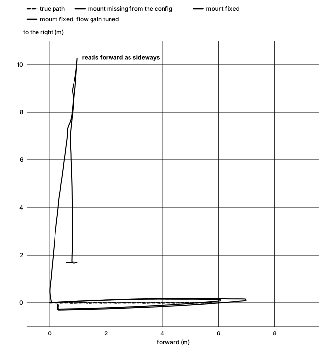
To tell whether it worked, I needed ground truth. The lab's motion capture tracks the robot more precisely than anything you could measure by hand, so I wrote the package that brings it into ROS: the EKF's estimate and the mocap pose land in one bag on one clock, and every run can be compared with the truth point by point. The first runs showed why that mattered: driving 5.5 m, the estimate stayed within 0.74 m of mocap, but spinning in place sent it 155 m off. Once teammates found the sensor's mounting missing from the config, I tuned the flow gain against mocap, run by run, until the estimate stayed within 5 mm of motion capture.

Top-down chart of a simulated drive: with the sensor's mounting missing from the config, the estimate heads 10 meters sideways while the robot drives 6 meters forward and back; with the mounting fixed, it follows the true path
In simulation (ArduPilot SITL, flow only, the sensor 10 cm off the floor): with the mounting missing from the config, driving forward reads as driving sideways.
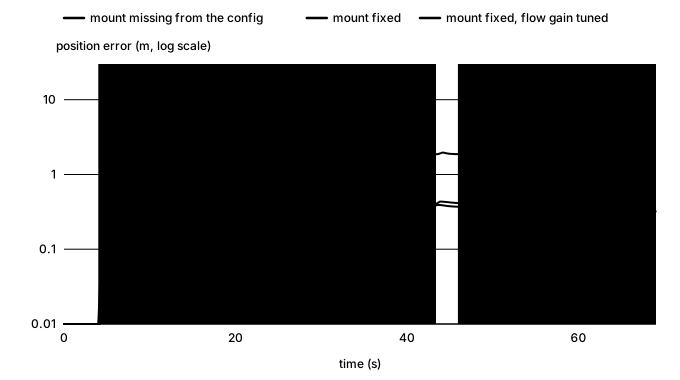
Chart of simulated position error over time for three configurations: mounting missing, up to about 11 meters; mounting fixed, about 1 meter; flow gain tuned, about half a meter
The same simulated run, error over time for each config. On the robot, against mocap, the tuned estimate stayed within 5 mm.