← All skills

Skill

Linear algebra

Vectors, matrices and spatial algebra. Achilles's own SIMD spatial algebra, and ARUW's Kalman filters split from 8×8 matrices into 2×2 ones.

4 log entries2 projects

AchillesBest example

SIMD: eight robots per instruction

Pull request

Also shows: Performance & SIMDC++

V3 replaces V2's Eigen with my own spatial algebra on xsimd, and stores every field as a structure of arrays: each component of each field, say the x angular velocity of every joint, is its own contiguous, aligned array. Joints are sorted by their depth in the tree, and each group of SIMD lanes holds joints at the same depth. With many copies of one robot, that puts the same joint of different robots side by side, so one instruction can load, update or store a quantity for eight robots at once (eight lanes with AVX2, four in the default SSE2 build). A Valgrind trace of the compiled binary confirms it: 88.9% of all accesses to simulation data are whole, aligned 8-lane vector loads or stores. The payoff is that filling the lanes is nearly free. On a seven-link arm, one robot takes 3.1 µs per step, while eight robots in the 8-lane build take 4.3 µs, 5.7× the robot-steps per second.
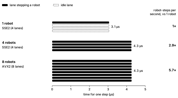
Three bars of SIMD lanes showing the time for one step of a seven-link arm: one robot in the 4-lane build takes 3.1 microseconds with three lanes idle; four robots fill the lanes in 4.3 microseconds, 2.9 times the robot-steps per second; eight robots in the 8-lane AVX2 build take 4.3 microseconds, 5.7 times
One step of a seven-link arm on one CPU core, best of 18 runs. Batched runs also step one shared fixed root.
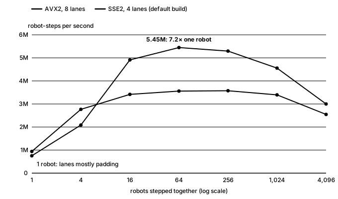
Line chart of robot-steps per second against robots stepped together, seven-link arm. With one robot, 8-lane AVX2 does 0.75 million and 4-lane SSE 0.94 million. AVX2 climbs to 5.45 million at 64 robots, 7.2 times its one-robot rate; SSE levels off near 3.6 million.
The same effect across batch sizes: throughput climbs until the lanes are full.

Achilles

Dynamics: the Articulated Body Algorithm

Pull request

Also shows: Kinematics & DynamicsC++Simulation (MuJoCo)

V2's dynamics were wrong in ways only a reference could show: brought back to life next to MuJoCo, a one-link arm swung exactly 4× too fast (it used the free-body inverse inertia, dropping the parallel-axis term), and a two-link arm moved in the wrong shape. V3 runs the full Articulated Body Algorithm, with Coriolis and centrifugal bias terms, parent-to-body transforms and gravity as a fictitious base acceleration, and steps it forward with semi-implicit Euler, the same default MuJoCo uses. Here all three drive the same arm with the same shoulder torque and no gravity, since V2 never had any. V3 stays within 3×10⁻⁵ rad of MuJoCo for all 4 seconds, while V2 has swung the shoulder 4.5 times as far and folded the elbow forward instead of letting it trail behind.

The demo arm with a constant 0.1 N·m on the shoulder, none on the elbow and no gravity, semi-implicit Euler at 1 ms. All three are drawn by MuJoCo's renderer, since V2 never had one; the yellow trail is the forearm tip's last second.

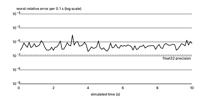
MuJoCo is only a reference, so I also checked V3 against an exact answer. A double pendulum is chaotic and has no closed-form trajectory: two simulations that differ by a single rounding error eventually go completely different ways. Its equations of motion do have a closed form, though. Lagrangian mechanics reduces them to a 2×2 linear system that gives the exact joint accelerations at any given position and velocity. I derived that system independently of the engine's code, then compared it with V3's accelerations at every state of a 10-second run. Because each state is checked on its own, errors can't build up and chaos can't amplify them. The two agree to within 3×10⁻⁶, which is float32 round-off, and V3 matches MuJoCo to the same 3×10⁻⁶.

Log-scale chart over 10 seconds of a double pendulum: the worst relative error in Achilles' joint accelerations against the closed-form solution stays between about 2e-7 and 3e-6, just above the float32 precision line, with no growth over time
ABA against the closed-form solution at every state of a 10-second double-pendulum run.

Advanced Robotics at UW

Kalman-filter odometry for three dead wheels

8-state filterSplit filters

Also shows: State estimationC++

Our robots know where they are from dead wheels: small unpowered tracking wheels with encoders that roll along the floor. When the engineer robot moved to new odometry pods with three of them, I rewrote the team's Kalman-filter odometry for them; I had taught myself Kalman filters from Kalman Filter from the Ground Up. The first version was one 8-state filter fusing the three wheels with the IMU. Its covariance between heading and the x and y motion turned out to be negligible, so I split it into three independent two-state filters, for x, y and heading, each updated by one measurement: every step now multiplies 2×2 matrices and divides by a number, instead of working through 8×8 matrices and inverting a 7×7 one, and the wheels alone turned out to be enough without the IMU. To tune it, I drove fixed paths (straight forward, straight sideways, spins and a square), logged the raw wheels, and replayed them offline to fit each pod's position, angle and wheel radius and the filter's noise, checking the result against the IMU's heading. Our target was under 10 cm of error over the engineer's path, the most our vision system could correct for, and the tuned odometry met it.

The engineer driving itself at competition, from the third cube pickup to its drop-off: the filter's own logged pose, replayed at real time from just before it moves.
Tuning offline: a logged 5 m sideways push, replayed through the filter as the pods move from their design values to the tuned ones. With one pod 2.7° off straight, the design values read the push as a 79° turn; tuned, it comes to 4.99 m and follows the path the IMU's heading gives, ending within 1° of it.

Advanced Robotics at UW

Path tracking: from pure pursuit to LQR

CodeThe LQR study

Also shows: Control systemsTechnical leadershipC++

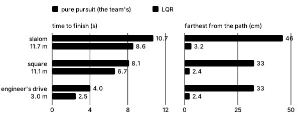
Our chassis followed paths with pure pursuit: aim at a point a fixed distance down the path and ramp the speed up toward it. The robot's accelerations stay implicit in that, so it has no idea how hard it can brake or how fast it can take a corner, and at speed it swings wide of turns and overshoots where it should stop. I proposed replacing it with path tracking that models those accelerations explicitly, and led the feature from idea to implementation: I wrote the design and gathered the resources behind it, from spline fitting and arc-length reparametrization to the Riccati equation and a study that found LQR tracks more accurately than pure pursuit. First, a cubic spline through the waypoints is reparametrized by arc length, the speed at each point is capped by its curvature, and a forward and a backward pass keep every speed-up and every stop within what the robot can deliver. Then an LQR tracks that profile on a world-frame model of the chassis, where its dynamics stay constant, and its force is rotated into the robot's frame. I designed it and built the framework; the comparison here runs the finished MVP against our pure pursuit in simulation.

The same slalom, the same simulated chassis and the same 2 m/s top speed: LQR (blue) against the team's pure pursuit (orange), in real time.
Bar charts for three paths: LQR finishes each sooner and stays within about 3 cm of the path, against 33 to 46 cm for pure pursuit
Three paths: LQR finishes 1.5 to 2.1 s sooner and stays within 3.2 cm of the path; pure pursuit strays up to 46 cm.