← All skills

Skill

Debugging

Tracking a failure to its cause. A singularity in the lab's IK solver, a missing sensor mounting that sent odometry 155 m off, and identical lidars on USB.

4 log entries2 projects

OpenDubsBest example

Fixing the IK solver for the OpenArm

The fixPull request

Also shows: Open sourceKinematics & DynamicsPython

Teleop and planning both lean on ssik, the lab's analytical IK solver, which I didn't write, and on the OpenArm it kept failing. I traced it to a singularity in the solver itself: the OpenArm's joint axes meet at shared points, so its link lengths are zero and every twist is a right angle, and that exact geometry breaks the Raghavan–Roth elimination the solver uses. My fix nudges those zero lengths by a tiny fraction of the arm's size, so the solver works on an arm a hair off the real one, then, since forward kinematics is cheap, refines the answer against the true arm's FK, step after step, until it's an exact solution again. The maintainer confirmed the fix would have worked while landing the same one upstream.
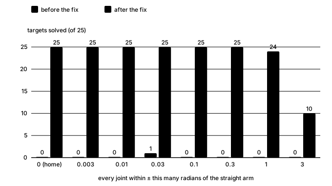
Bar chart of IK targets solved on the OpenArm, 25 per distance from the straight arm, from 0 to 3 radians: before the fix, 1 of 200 in all; after it, every target out to 0.3 radians, 24 at 1 radian and 10 at 3
My July OpenArm IK (ssik's joint-lock solver) on 200 random reachable targets, run again with ssik just before my fix and with it: 1 solved before, 184 after.

OpenDubs

Optical flow odometry, checked against mocap

micro-ROS bridgeMocap package

Before the base could navigate, it had to know where it was. The first source was optical flow: a sensor that watches the floor slide past. I brought it up over micro-ROS and fed it into ArduPilot's EKF alongside the IMU of the Pixhawk the base ran at the time. It only read sensibly within about 10 cm of the floor, so it sits low, lit by its own LED.

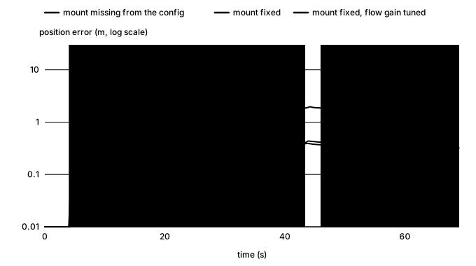
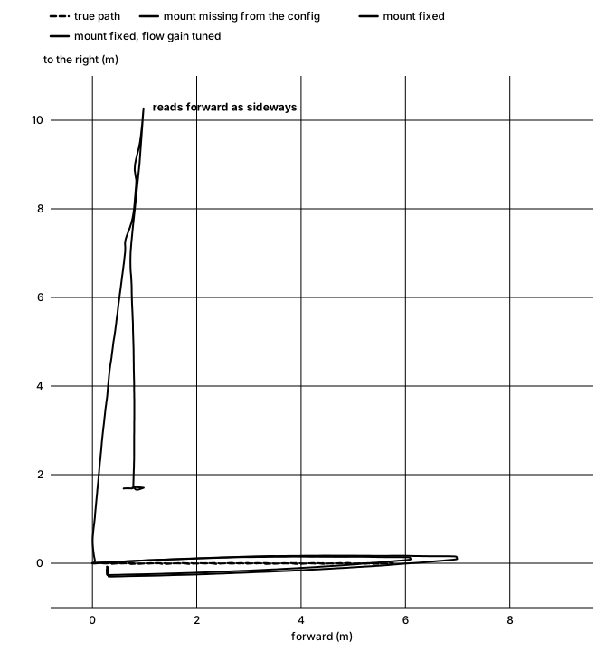
To tell whether it worked, I needed ground truth. The lab's motion capture tracks the robot more precisely than anything you could measure by hand, so I wrote the package that brings it into ROS: the EKF's estimate and the mocap pose land in one bag on one clock, and every run can be compared with the truth point by point. The first runs showed why that mattered: driving 5.5 m, the estimate stayed within 0.74 m of mocap, but spinning in place sent it 155 m off. Once teammates found the sensor's mounting missing from the config, I tuned the flow gain against mocap, run by run, until the estimate stayed within 5 mm of motion capture.

Top-down chart of a simulated drive: with the sensor's mounting missing from the config, the estimate heads 10 meters sideways while the robot drives 6 meters forward and back; with the mounting fixed, it follows the true path
In simulation (ArduPilot SITL, flow only, the sensor 10 cm off the floor): with the mounting missing from the config, driving forward reads as driving sideways.
Chart of simulated position error over time for three configurations: mounting missing, up to about 11 meters; mounting fixed, about 1 meter; flow gain tuned, about half a meter
The same simulated run, error over time for each config. On the robot, against mocap, the tuned estimate stayed within 5 mm.

OpenDubs

Two 2D lidars, merged into one scan

Also shows: State estimationROS 2Hardware bring-upPython

For localization and a map, the base carries two RPLIDAR A1 2D lidars, one at the front and one at the back. Bringing them up, with the team, was mostly fighting USB: the two units have identical USB IDs, so udev rules name each by the hub port it's plugged into, and they power up a few seconds apart so neither times out.

Mapping and Nav2 expect one scan, so I wrote a node that merges the two. The two scans never line up on their own: nothing guarantees the lidars spin at exactly the same rate or finish a revolution at the same moment, and each reaches the Thor with its own latency. So the node pairs scans by their timestamps (any two within 0.1 s), looks up each scan's transform into the robot's frame at that scan's own timestamp, resamples both to the finer of the two angular resolutions, and keeps the nearest return in each direction of one 360° scan, stamped halfway between the two and dropping hits on the robot itself. On top of it, I set up slam_toolbox and Nav2, which drove the robot point to point in simulation.

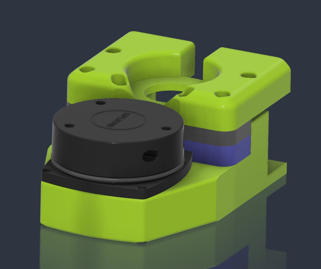
A CAD render of a round 2D lidar sitting in a bright green 3D-printed mount
One of the two lidar mounts. CAD render from the lab's build guide.
A replay in Gazebo: the robot's URDF, my lidar merger and our slam_toolbox settings, unmodified, mapping a made-up lab room while Nav2 drives. 6× speed.

Achilles

Dynamics: the Articulated Body Algorithm

Pull request

Also shows: Kinematics & DynamicsC++Simulation (MuJoCo)

V2's dynamics were wrong in ways only a reference could show: brought back to life next to MuJoCo, a one-link arm swung exactly 4× too fast (it used the free-body inverse inertia, dropping the parallel-axis term), and a two-link arm moved in the wrong shape. V3 runs the full Articulated Body Algorithm, with Coriolis and centrifugal bias terms, parent-to-body transforms and gravity as a fictitious base acceleration, and steps it forward with semi-implicit Euler, the same default MuJoCo uses. Here all three drive the same arm with the same shoulder torque and no gravity, since V2 never had any. V3 stays within 3×10⁻⁵ rad of MuJoCo for all 4 seconds, while V2 has swung the shoulder 4.5 times as far and folded the elbow forward instead of letting it trail behind.

The demo arm with a constant 0.1 N·m on the shoulder, none on the elbow and no gravity, semi-implicit Euler at 1 ms. All three are drawn by MuJoCo's renderer, since V2 never had one; the yellow trail is the forearm tip's last second.

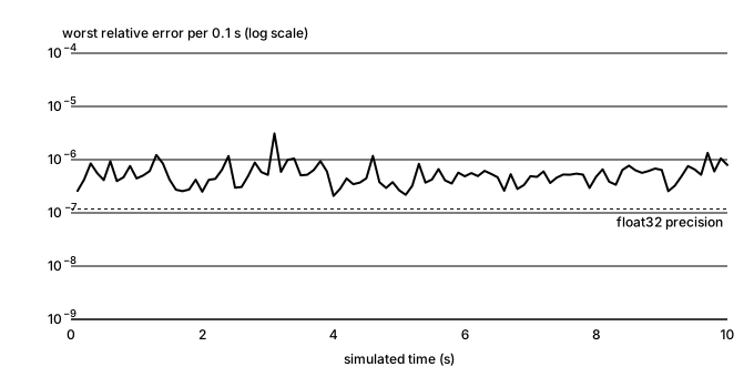
MuJoCo is only a reference, so I also checked V3 against an exact answer. A double pendulum is chaotic and has no closed-form trajectory: two simulations that differ by a single rounding error eventually go completely different ways. Its equations of motion do have a closed form, though. Lagrangian mechanics reduces them to a 2×2 linear system that gives the exact joint accelerations at any given position and velocity. I derived that system independently of the engine's code, then compared it with V3's accelerations at every state of a 10-second run. Because each state is checked on its own, errors can't build up and chaos can't amplify them. The two agree to within 3×10⁻⁶, which is float32 round-off, and V3 matches MuJoCo to the same 3×10⁻⁶.

Log-scale chart over 10 seconds of a double pendulum: the worst relative error in Achilles' joint accelerations against the closed-form solution stays between about 2e-7 and 3e-6, just above the float32 precision line, with no growth over time
ABA against the closed-form solution at every state of a 10-second double-pendulum run.